Bloom filters are a data structure which allows you to test whether an element exists in a set, with lower memory usage and better access times than other hash table implementations. It is probabilistic, and while it can guarantee negative matches, there is a slight chance it returns a false positive match. Through clever mathematical assumptions, we can produce constraints to minimise the chance of a false positive.
Contents
Description
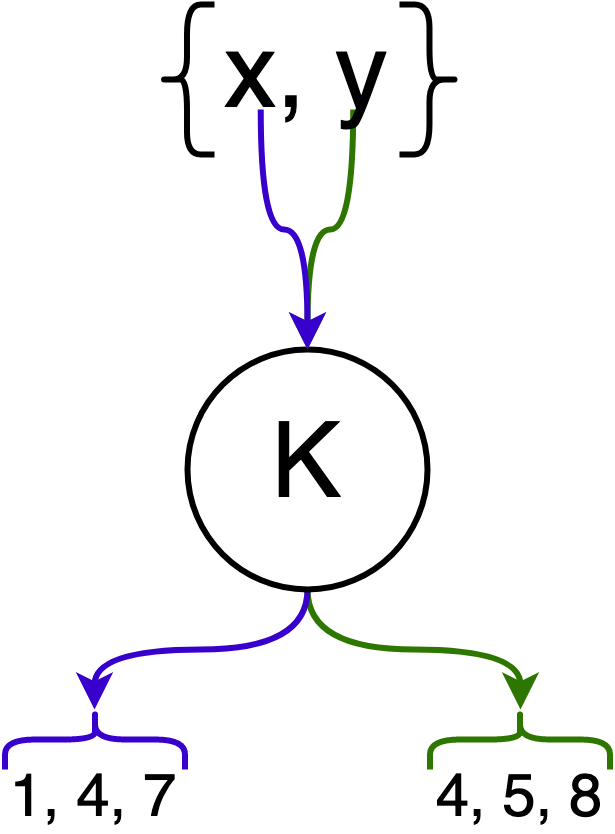
Let there be a set of elements $N$, and we wish to store each element $e \in N$ in the set $F$. To do this, we introduce the set $K$ which has $k$ number of hash functions which hash the same element to different values.
In the following example, elements $x$ and $y$ are hashed by $k = 3$ hash functions.
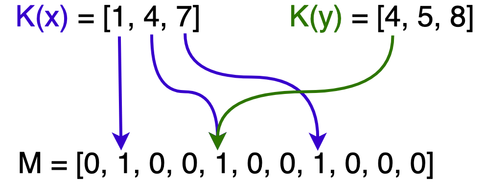
Next, we introduce the bit array $M$ which has $m$ bits. This bit array is the underlying data structure that represents $F$, and we say an element $e$ is in $F$ if all of its corresponding bits (after hashing) in the bit array are set.
In the following image, $x$ is in $F$ hence all of its hashed bits within $M$ are set. Only one of $y$’s hashed bits are set so it is not in $F$. $x$ and $y$ are also sharing a bit at $M[4]$.
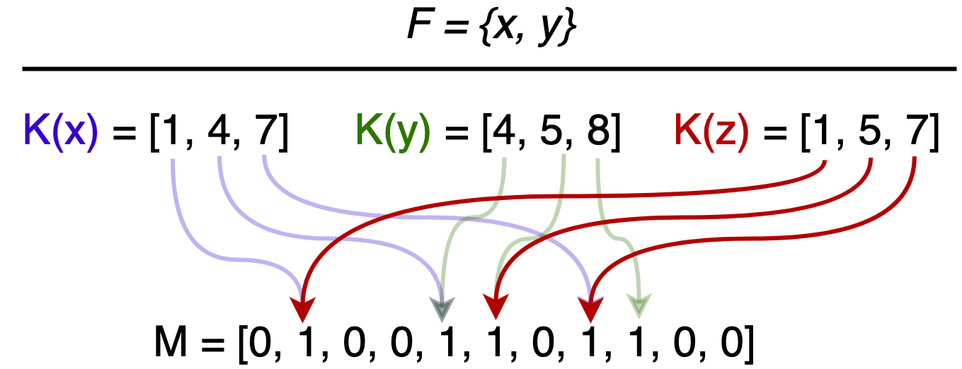
As we hash more elements from $N$, more bits are set to 1 in $M$ and eventually we get a false positive when testing set membership. This occurs when all of an element’s bits are set, although it was never inserted.
Consider the following scenario: $x$ and $y$ are in $F$, $z$ is not. However, $z$’s hashed bits are all set, giving the (false) impression that $z$ is in $F$.
Once an element is placed in $F$, it will remain there, as flipping bits to remove an element introduces the possibility of false negatives. We will show that there exists optimal parameters, $k$ hash functions and $m$ length bit array, to lower the false positive rate $\epsilon$.
Proof
Note: This section is pretty math heavy, if you just want to look at the cool tables and graphs then you can skip ahead to here.
$\newcommand{\pbrac}[1]{\left(#1\right)}$ $\newcommand{\sbrac}[1]{\left[#1\right]}$
First attempt
Assume that a hash function in $K$ maps to each array position with equal probability. The probability that a bit is not set by a hash function during the insertion of an element is:
\begin{align} 1 - \frac{1}{m}. \end{align}
The probability that every hash function in $K$ leaves a certain bit at 0 will be
\begin{align} \left( 1 - \frac{1}{m} \right)^k \approx \ e^{-k/m}. \end{align}
Thus, after inserting $n$ elements, the probability that a bit is still 0 is
\begin{align} \left( 1 - \frac{1}{m} \right)^{kn} \approx \ e^{-kn/m} \ = \ p, \end{align}
and the probability that a bit is 1 after $n$ insertions is
\begin{align} \left( 1 - \left[ 1 - \frac{1}{m} \right]^{kn} \right) \approx \left( 1 - p \right). \end{align}
Next, we test set membership for an element NOT in the set. Following $n$ insertions, each bit in the array has a chance of being set to 1 with the probability above. The probability that $k$ bits are set to 1, which would lead to a false positive result for set membership, is often referred to as the error/false positive rate:
\begin{align} \epsilon = \left( 1 - \left[ 1 - \frac{1}{m} \right]^{kn} \right)^k \approx \left( 1 - p \right)^k. \end{align}
There exists a major problem with this analysis, however. At the start we made an assumption that all bits would be set randomly and independently. This is not correct as we have established that all our hash functions in $K$ will not hash an element to the same array position. For example, if we have hashed an element $m-1$ times into $m-1$ different positions, then the remaining $1$ bit in the array is guaranteed to be chosen, if we wish to retain an even spread of hashed values. Concretely, the $k$ bit array positions for each element are in fact dependent.
Another try using Poisson approximations
Consider a “balls and bins” scenario where each throw of a ball into a bin is equivalent to hashing an element to an array position.
We have the following 2 cases:
- Exact case: $n$ balls are thrown into $m$ bins independently and uniformly at random
- Poisson case: number of balls in each bin are taken to be independent Poisson random variables with an expected value
We’ll be using the following corollaries from the book “Probability and computing: randomization and probabilistic techniques in algorithms and data analysis” by Mitzenmacher and Upfal.
Corollary 4.6: Let $X_1,…,X_n$ be independent Poisson trials such that $P(X_i = 1) = p_i$. Let $X = \sum_{i=1}^{n} \text{ and } \mu = E(X)$. For $0 < \delta < 1$. [p. 71] \begin{align} P\left(\left|X - \mu\right| \geq \delta \mu\right) \leq 2\exp{\left(-\frac{\mu\delta^2}{3}\right)} \end{align}
Corollary 5.9: any event that takes place with probability $p$ in the Poisson case takes place with probability at most $p e \sqrt{n}$ in the exact case. [p. 109]
Each bin corresponds to an array position and thus a bit being set to 0 is equivalent to an empty bin in our scenario. The fraction of bits being set to 0 after $n$ insertions is therefore equivalent to the fraction of empty bins after $kn$ balls have been thrown into $m$ bins.
We define $X$ as the number of empty bins after the balls have been thrown into $n$ bins, such that
\[\begin{align} X =& \ \sum_{i=1}^{n} X_i, \\ \text{where } X_i =& \ \begin{cases} 1 & \text{if bin is empty} \\ 0 & \text{otherwise} \end{cases} \end{align}\]then we can define
\[\begin{align} p' =& \ \left( 1 - \frac{1}{m}\right)^{kn}, \\ E(X) =& \ mp'. \end{align}\]In the Poisson case, each bin can be thought of as an independent Poisson random variable with expected value $p’$. Therefore, we can apply \textbf{corollary 4.6} and $E(X) = \ mp’$ to obtain the following:
\begin{align} P\left( \left| X - mp’\right| \geq \delta mp’\right) \ \leq& \ 2\exp{\left(-\frac{mp’\delta^2}{3}\right)} \end{align} Let $\delta \ = \ \beta / p’, \ $choose small$ \ \beta$ \begin{align} \therefore \ P\left( \left| X - mp’\right| \geq \beta m\right) \ \leq& \ 2\exp{\left(-\frac{m\beta^2}{3p’}\right)} \end{align}
We then apply corollary 5.9 to obtain
\[\begin{align} P\left( \left| X - mp'\right| \geq \beta m\right) \ \leq& \ 2e\sqrt{kn} \exp{\left(-\frac{m\beta^2}{3p'}\right)}\\ \leq& \ 0.000001 \ \text{when $m$ sufficiently large.} \end{align}\]Essentially, taking the probability of an event using a Poisson approximation for all of the bins and multiplying it by $e\sqrt{kn}$ gives an upper bound for the probability of the event when $kn$ balls are thrown into $m$ bins (the exact case where events are independent).
This result tells us that when $m$ is sufficiently large, the fraction of empty bins $X/m$ is very close to $p’$. And since $p’ \approx p$ we can use $p$ to continue predicting actual performance.
Optimal k
The false positive rate is $\epsilon = (1-p)^k$ and we look for a $k$ that minimizes $\epsilon$. Rearranging $\epsilon$ gives us
\[\begin{align} \epsilon \ =& \ \pbrac{1-p}^k \\ =& \ \exp{\pbrac{\ln{\pbrac{\sbrac{1-p}^k}}}} \\ =& \ \exp{\pbrac{k\ln{\pbrac{\sbrac{1-p}}}}} \\ =& \ \exp{\pbrac{k\ln{\pbrac{\sbrac{1-e^{-kn/m}}}}}}. \end{align}\]If we let $g = k\ln{\pbrac{1-e^{-kn/m}}}$ so that $\epsilon = e^g$, then minimizing the false positive $\epsilon$ is equivalent to minimizing $g$ with respect to $k$. We have
\begin{align} \frac{dg}{dk}\ =& \ \ln \left(1-e^{-\frac{nk}{m}}\right)+\frac{kn \cdot e^{-\frac{nk}{m}}}{m\left(1-e^{-\frac{nk}{m}}\right)}. \end{align}
Solving this derivative when it is 0 and finding the global minimum gives us
\begin{align} k = \frac{m}{n}\ln\pbrac{2}. \end{align}
Optimal m
To find an optimal length for our bit-array we substitute $k = \frac{m}{n}\ln\pbrac{2}$ into our false positive equation and get
\[\begin{align} \epsilon \ =& \ \pbrac{1-e^{-\ln 2}}^{\frac{m}{n}\ln 2} \\ \ln\epsilon \ =& \ \frac{m}{n}\ln\pbrac{2}\ln\pbrac{1-e^{-\ln 2}} \\ =& \ \frac{m}{n}\ln\pbrac{2}\ln{\frac{1}{2}} \\ =& \ -\frac{m}{n}\ln\pbrac{2}^2 \\ \therefore m \ =& \ \frac{-n\ln\epsilon}{\ln\pbrac{2}^2}. \end{align}\]This effectively leaves $\epsilon$ as the only unknown variable left. However, when we consider the Bloom filter in a practical context, we will most likely have a false positive rate in mind, and can treat it as a constant.
Implementation and benchmarks
Overview
We will be comparing the Bloom filter against 4 popular and efficient implementations of hash tables:
- Google Dense Hash Set
- Google Sparse Hash Set
- TSL Robin Set
- STD Unordered Set
Implementations were compared based on time performance (insert, read) and memory performance (inserts). Currently, only small strings (15 characters) and medium strings (50 characters) are used for input, with up to $n = 3\times10^6$ elements for each test. Each test was performed 5 times for each implementation and an average-of-5 was used in the final table/graph. The false positive rate is set to 0.01.
Benchmarking was done using gcc’s C++ compiler and the following command was run to compile: g++ -Iinclude -std=c++11 -O3. In addition, the tests were performed on a computer with the following specs:
- AMD Ryzen 5 2600 3.4GHz 6 core
- 8GB DDR4-2666 CL19
The tests were run with the false positive rate $\epsilon = 0.01$
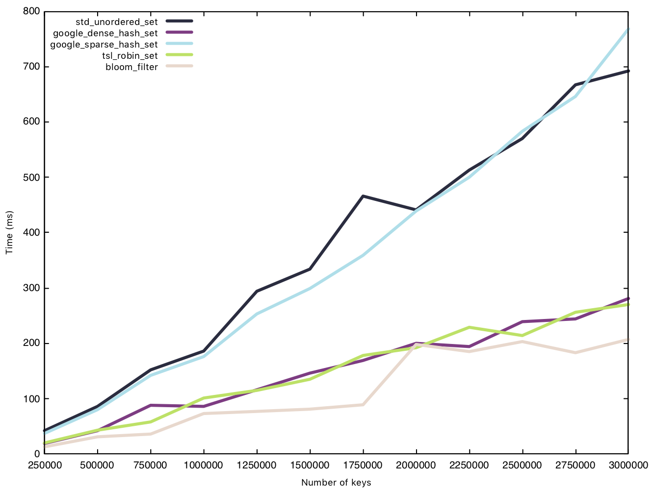
Insert small string (15 bytes)
Before the test, we generate a vector of $n$ small strings and then insert each string as an entry into the sets, measuring the performance of said insert operation. The Bloom filter’s only overhead during insertion is setting bits to 1.
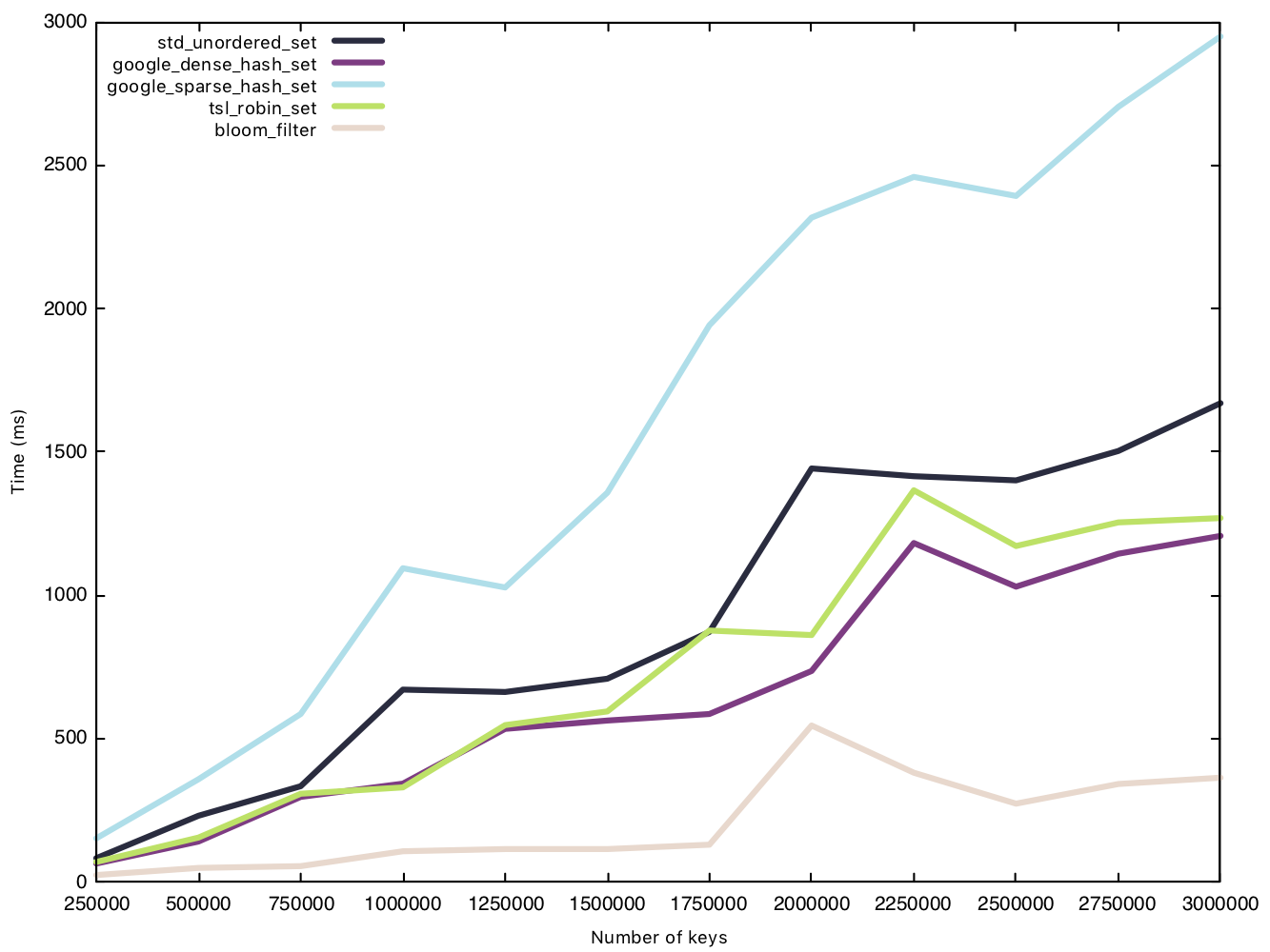
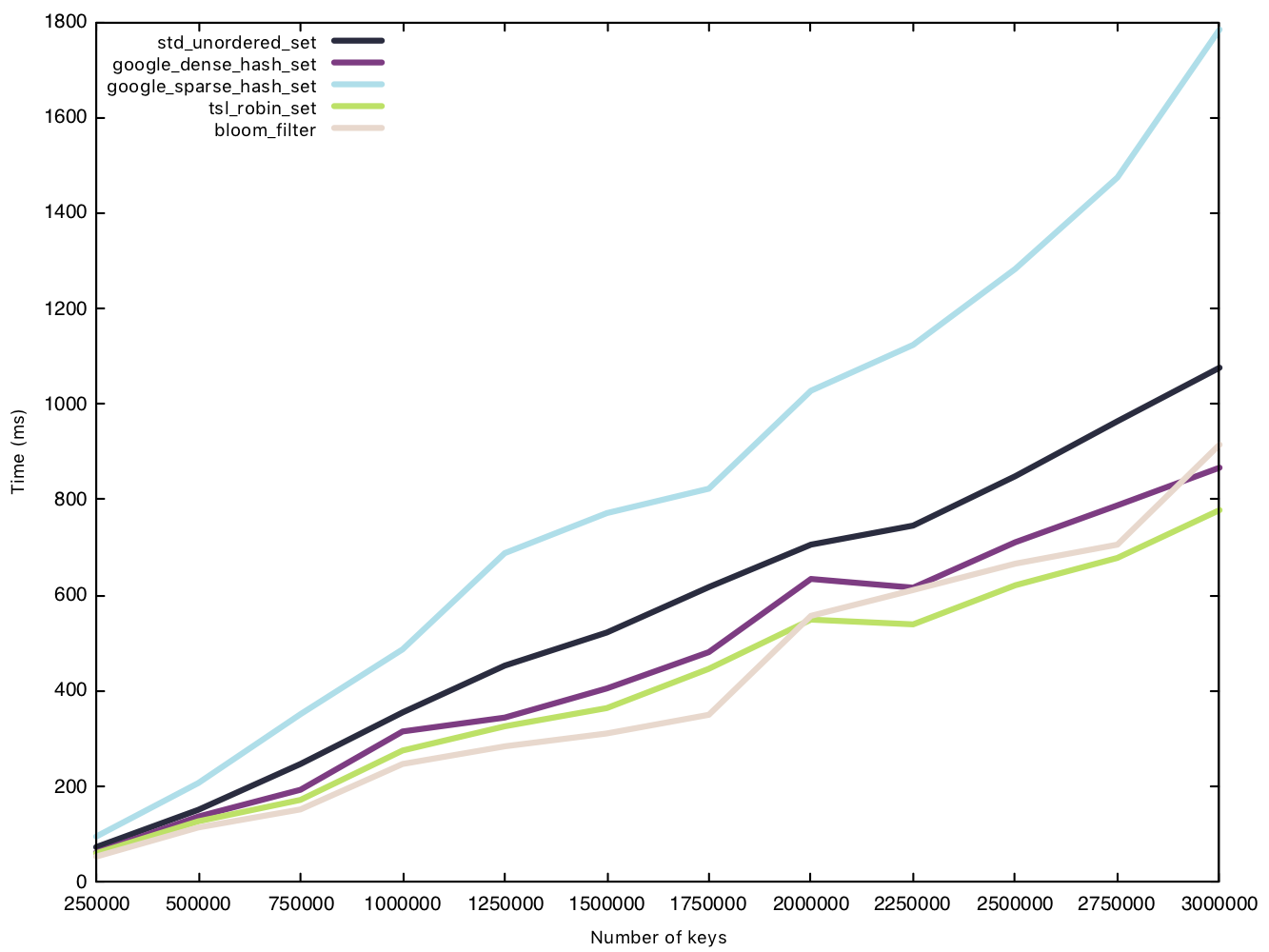
Read small string (15 bytes)
Before the test, we generate a vector of $n$ small strings and pre-load the strings into the hash tables. We then traverse the same vector of small strings, testing set membership and timing said read operation.
From our results, the sparsehash and std implementation perform almost equally, but not quite as fast as our other implementations. While the Bloom filter was the clear winner in our insertion battle, its victory is marginal when it comes to read operations
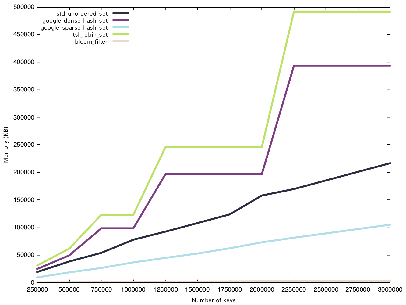
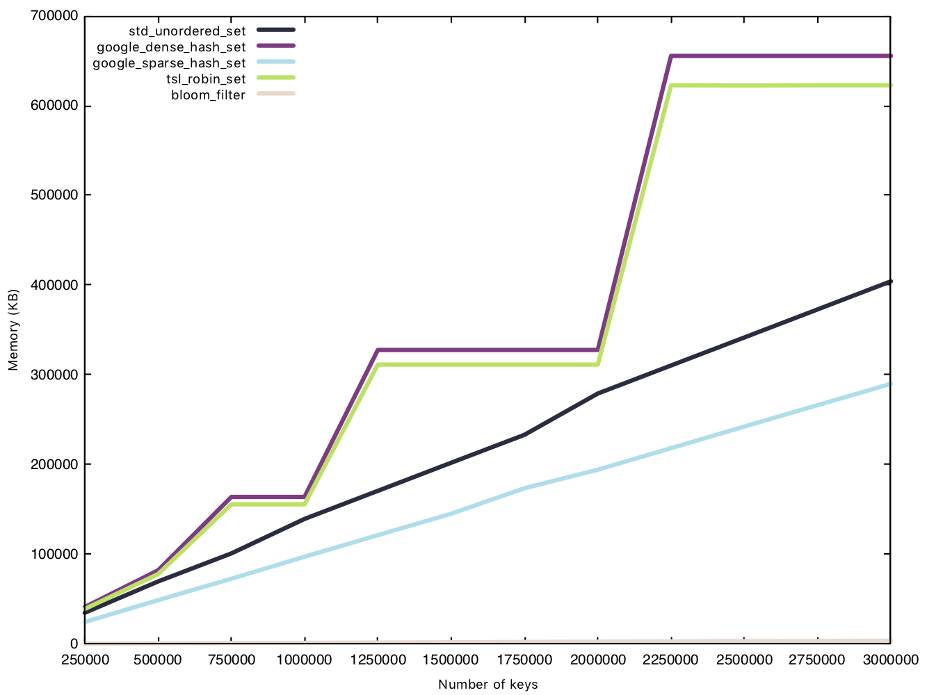
Memory usage - small string (15 bytes)
This test is conducted in the same manner as the insertion test, except we measure memory usage before and after the $n$ insertions. Because the Bloom filter’s memory overhead is determined before operations, we will consider them in our data for a fair comparison.
This is where the Bloom filter stands out, as a space efficient data structure. sparsehash, a memory efficient hash table in its own right, can only manage a 216MB overhead with 3 million elements, while our Bloom filter remains under 4MB, that’s 1% of sparsehash’s memory usage! Amazing!
Two implementations have rather funky lines on the graph, densehash and robin_set, as they grow in what’s called a “power-of-2” growth policy, where the number of “bins” is rounded up to the next power of 2, as bitwise modulo for powers of 2 are faster than regular modulo operations.
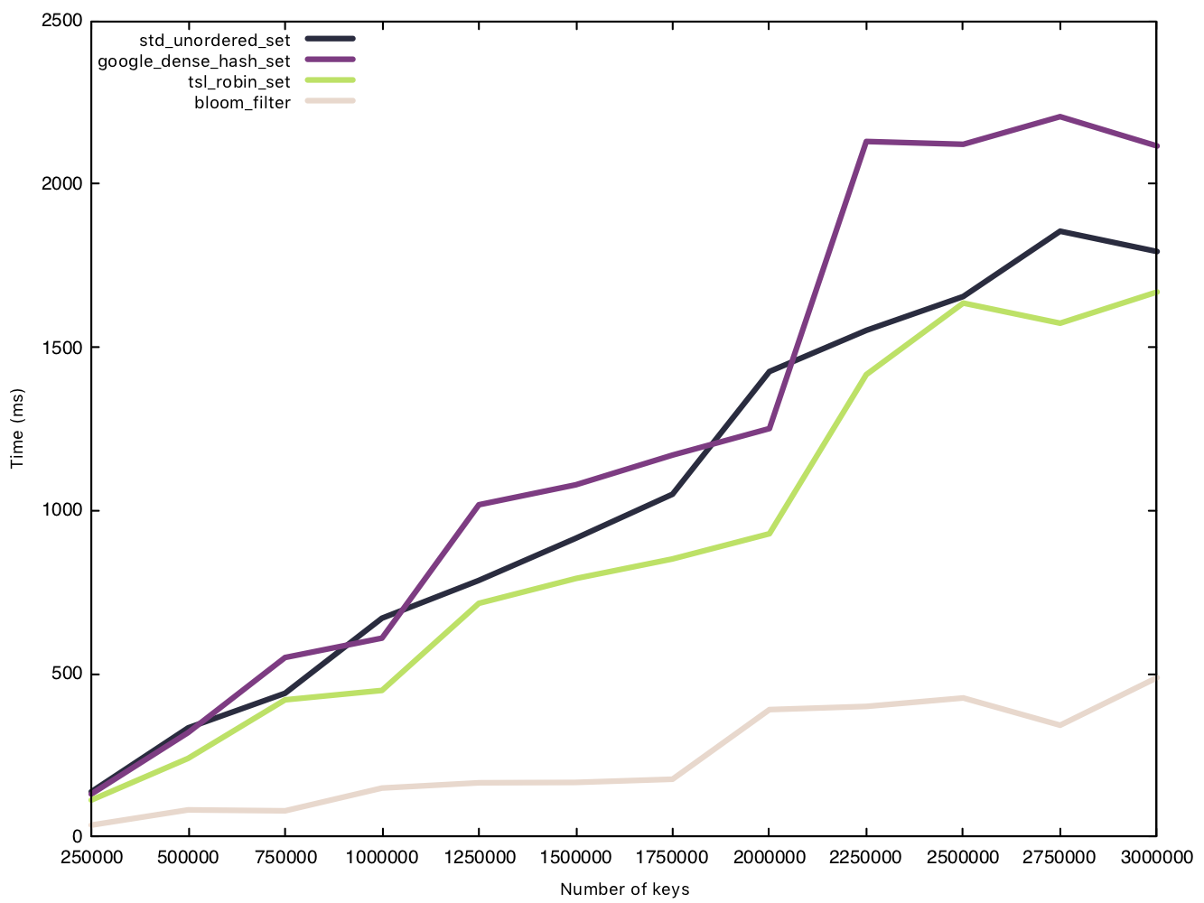
Insert string (50 bytes)
When handling bigger strings, the other implementations see a very obvious increase to the time taken to insert all $n$ elements. The Bloom filter, however, takes nearly the exact same amount of time (increasing slightly due to the hash function having to hash a bigger string), and remains under the 500ms mark. The size of the element makes no difference to the Bloom filter bookkeeping overhead.
Read string (50 bytes)
Read operations, again, prove to be the great equaliser, and we see a very tight cluster of times except for sparsehash, which separates itself from the pack. In our first comparison of read operations, sparsehash and the std implementation were equal in performance. With bigger strings, however, the std implementation is the clear winner.
Memory usage - string (50 bytes)
Once again, the Bloom filter performs spectacularly. In fact, it uses the same memory overhead as it did in the 15 bytes memory test. Earlier we showed that $m$, the amount of bits in our bit array, is on conditioned $n$. Meaning even if the elements we were hashing got larger, our memory overhead would remain the same. This is quite useful as it allows us to hash relatively long strings (e.g. URLs) with no extra space used compared to a smaller string.
Furthermore, it is clear the reason sparsehash performs so badly in our insertions is because it takes extra steps to reduce space usage. We also see densehash and robin_set repeating the same behaviour in the earlier test, utilising the same “power-of-2” growth policy.
False positives - is the math accurate?
We now test the false positive rate for the Bloom filter. The methodology is as follows: insert $n$ strings into the Bloom filter, generate $n$ new strings NOT currently in the set, and check set membership. We then count the number of times a false positive occurs. In this test we will set $\epsilon = 0.01$.
In the following tables, we see that the false-positive rates for both small and normal strings are very, very close to the value we set, 0.01. We can safely work with Bloom filters with the assumption that false-positives only occur at a rate of $\epsilon$.
Small strings (15 bytes)
| n | false-positives | false-positive rate |
|---|---|---|
| 250000 | 2526 | 0.010104 |
| 500000 | 4974 | 0.009949 |
| 750000 | 7527 | 0.010037 |
| 1000000 | 10078 | 0.010078 |
| 1250000 | 12633 | 0.010107 |
| 1500000 | 14982 | 0.009988 |
| 1750000 | 17639 | 0.010080 |
| 2000000 | 20165 | 0.010082 |
| 2250000 | 22709 | 0.010093 |
| 2500000 | 25027 | 0.010011 |
| 2750000 | 27600 | 0.010037 |
| 3000000 | 30153 | 0.010051 |
Strings (50 bytes)
| n | false-positives | false-positive rate |
|---|---|---|
| 250000 | 2544 | 0.010178 |
| 500000 | 5061 | 0.010124 |
| 750000 | 7462 | 0.009950 |
| 1000000 | 9967 | 0.009967 |
| 1250000 | 12526 | 0.010021 |
| 1500000 | 15093 | 0.010062 |
| 1750000 | 17569 | 0.010040 |
| 2000000 | 20035 | 0.010018 |
| 2250000 | 22621 | 0.010054 |
| 2500000 | 25053 | 0.010022 |
| 2750000 | 27531 | 0.010012 |
| 3000000 | 30062 | 0.010021 |
Example usage scenario
Consider a web browser that has the feature to alert users about suspicious URLs. When it spots a suspicious URL, it runs a full diagnostic check on the website first before allowing the user to proceed. Using a Bloom filter, we can create a set of suspicious URLs that takes up minimal space on a server or in memory. Every time a user visits a URL, the browser can preempt the user and check to see if the URL is currently in the set of suspicious URLs. If the site is indeed suspicious, the browser runs a diagnostic check. If the site is not suspicious but there is a false positive, then the browser still runs the diagnostic check. Even if false positives occur, this is a worthy trade-off as we have saved space and reduced the time it takes to check a URL.